Multiple linear regression in a distributed system
Adapting a multiple linear regression algorithm for distributed computation.
In a previous post I talked about adapting a linear regression algorithm so it can be used in a distributed system. Essentially, a master computer oversees computations run on local data, and the algorithm pauses midway through to send summary statistics to the master. In this way, the master receives enough information to reconstruct the model without seeing the underlying data.
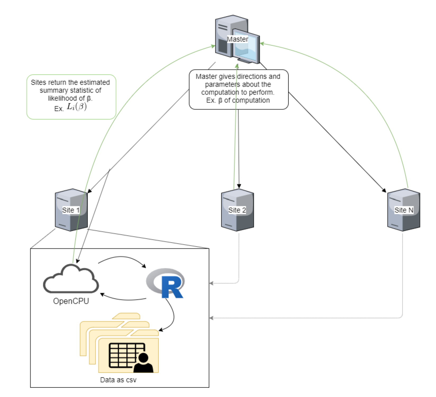
For a linear regression model, we can simply have the master iteratively pass candidate \(\beta\)s values to to the workers, which then return their local sum of the residual squares. By minimizing the sum of the squared residuals on each iteration, the master can find the optimal values for the \(\beta\)s in \(y=\beta_0 + \beta_1x\).
We can expand this from simple linear regression with a single predictor to multiple linear prediction with several predictors ($y=\beta_0 + \beta_1x + … +\beta_nx$). The sum of the squared residuals is simply the summary statistic of a matrix operation. Therefore a master controller can pass a vector of \(\beta\) parameters to the workers on each iteration and receive the RSS in return:
$$RSS_{local}=\sum_{i=1}^n{\begin{bmatrix}
 x_{1,1} & ... & x_{1,n} & \\
 ... & ... & ... & \\
 x_{m,1} & ... & x_{m,n} &
 \end{bmatrix}\times\begin{bmatrix}
 \beta_0 \\
 ... \\
 \beta_m
 \end{bmatrix}}$$
With a few minor changes in code from my previous post, we can adjust our loss function to accomodate a vector of \(\beta\)s.
# define a residual sum of squares function to handle multiple sites
multi.min.RSS <- function(sites, par){
  rs <- 0
  # calculate the residuals from each data source
  for(site in sites){
    tmp_mat <-as.matrix(site$data[,1:(ncol(site$data)-2)])
    tmps <- par[1] + tmp_mat%*%par[-1] - site$data$y
    rs <- rs + sum(tmps^2)
  }
  # return the square and sum of the residuals
  return(rs)
}
Now all we need to do is simulate some multi-variate data and test everything out.
# general function for simulating a sample data set given parameters
sim.data <- function(mu, sig, amt, seed, mpar, nl){
  # Simulate data for the practice
  set.seed(seed)
  x <- replicate(length(mpar)-1, rnorm(n=amt, mean=mu, sd=sig))

  # create the "true" equation for the regression
  a.true <- mpar[-1]
  b.true <- mpar[1]
  y <- x%*%a.true+b.true

  # set the noise level
  noise <- rnorm(n=amt, mean=0, sd=nl)
  d <- data.frame(x
                  , "y_true"=y
                  , "y"=y + noise)
  return(d)
}

true_vals <- c(2,4,6,8)

sim.data1 <-sim.data(10,2,100,2020,true_vals,1)
sim.data2 <- sim.data(10,2,100,2019,true_vals,1)
sites <- list(site1 = list(data=sim.data1), site2 = list(data=sim.data2))

knitr::kable(head(sim.data1))
| X1 | X2 | X3 | y_true | y |
|---|---|---|---|---|
| 10.753944 | 6.542432 | 8.540934 | 152.5978 | 153.5145 |
| 10.603097 | 8.017478 | 11.702755 | 186.1393 | 185.9124 |
| 7.803954 | 8.828989 | 9.207017 | 159.8459 | 161.0281 |
| 7.739188 | 10.767043 | 10.813357 | 184.0659 | 185.5874 |
| 4.406931 | 11.493330 | 7.922893 | 151.9708 | 153.4088 |
| 11.441147 | 8.143158 | 7.488237 | 156.5294 | 158.8567 |
knitr::kable(head(sim.data2))
| X1 | X2 | X3 | y_true | y |
|---|---|---|---|---|
| 11.477045 | 8.309900 | 11.441690 | 189.3011 | 189.1410 |
| 8.970479 | 11.715855 | 9.210739 | 181.8630 | 181.7065 |
| 6.719637 | 8.632787 | 11.965325 | 176.3979 | 177.0496 |
| 11.832074 | 9.978611 | 7.191396 | 166.7311 | 167.2667 |
| 7.465036 | 7.191671 | 11.600407 | 167.8134 | 168.0076 |
| 11.476496 | 12.783553 | 8.498515 | 192.5954 | 192.8948 |
We can test our loss function with a call to optim and compare the results to the base R linear modeling function (and the true values of our simulation).
param.fit <- optim(par=c(0,0,0,0),
                   fn = multi.min.RSS,
                   hessian = TRUE,
                   sites=sites)

# stack the data frames vertically for later verification
sim.data3 <- as.data.frame(rbind(sim.data1, sim.data2))
mlm <- lm(y~., data=sim.data3[,-4])

d <- data.frame("True Betas"=true_vals
           , "Base R Coefficients"=coef(mlm)
           , "Distributed Coefficients"=param.fit$par)
knitr::kable(d)
| True.Betas | Base.R.Coefficients | Distributed.Coefficients | |
|---|---|---|---|
| (Intercept) | 2 | 2.604539 | 2.642250 |
| X1 | 4 | 4.018984 | 4.021583 |
| X2 | 6 | 5.936988 | 5.935438 |
| X3 | 8 | 7.978939 | 7.973534 |
Not far off!
You can run the full code here.